Event planning during COVID-19
“Hey, don’t come around here no more.” “So tonight I’m gonna party like it’s 1999.”
When considering whether to host or attend a gathering during the pandemic, it is helpful to have an idea about how risky the event is. One important aspect of this assessment is the probability that someone at the event will be unknowingly contagious with COVID-19. To help with this analysis, we have put together an interactive dashboard that will provide the estimated probability that someone at the event will be contagious with COVID-19 based on the number of guests and location.
More People, More Probability
Some people say “mo’ money, mo’ problems”, but with Covid-19 “mo’ people, mo’ probability” is more accurate. The more people at an event, the more likely at least one person is unknowingly infected and contagious. Figure 1 show the probability that someone at an event is infected as a function of the number of people at the event and the percent of people in the region that are infected. At the time of writing, roughly 1% of the US is estimated to be unknowingly infected with COVID-19. This means that there is a 25% chance that someone is unknowingly infected (and contagious) in a gathering of 29 people randomly selected from the US.
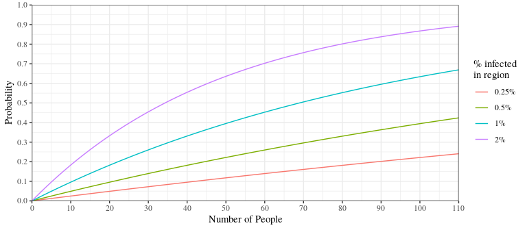
Figure 1: Probability that at least one person at an event is infected.
To help calculate the probabilities, we use the Complement Rule from probability theory: the probability that at least one person is infected is one minus the probability that no one is infected. If \(p\) is the proportion of a region that is infected, then \((1-p)^n\) is the probability that \(n\) randomly selected people from that region are all uninfected. And \(1-(1-p)^n\) is then the probability that at least one of the \(n\) people is infected.
To be more accurate, since we are dealing with finite population and sampling without replacement, the number of people that are infected in a region more closely follows a hypergeometric distribution. More details of the actual calculations are provided in the Details Section.
Estimating the number of unknowingly contagious in a population
We want to estimate the probability that someone at the event is unknowingly contagious. We use the term unknowingly because if anyone knows or suspects they are infected, we expect they will not attend. This implies that we want to estimate the likelihood that a person coming from a certain location is contagious, but either asymptomatic (won’t ever have any COVID-19 symptoms) or pre-symptomatic (will eventually get one or more COVID-19 symptoms). A major complication is that we don’t actually know how many people are infected at a given location and time, but only have data (and forecasts) about those that have been tested. To help us estimate the desired probabilities, we are using the CDC’s planning report.
This requires estimating three components: i) the actual number of infected people from the observed positive tests (case counts), ii) the number of the infected, but asymptomatic, people who weren’t tested, and iii) the number of those that will be contagious during the event date. We describe each of these in turn.
Estimating the Actual Infections
Our first step is to estimate the actual number of infected people from the observed positive test data. We know that the actual number infected is greater than the positive test data; let’s say the actual number of infected people in a region will be roughly \(r\) times the number of reported positive tests (with \(r>1\)). That is, if there are \(C_t\) people who have a positive test on day \(t\), there are actually \(rC_t\) people that would have had a positive test if they were tested. There are many reasons why people aren’t tested: they are asymptomatic and don’t know they are infected, they have mild symptoms and don’t want to bother with the time and expense of getting tested, they strongly suspect they are infected (e.g., one person in their household tested positive), testing isn’t available in their region, etc. It is also possible that an infected person is tested, but receives a negative result (i.e., false negative).
What value should we use for \(r\)? We have a few resources to guide us. First, the CDC cites a publication that compared the number of people with COVID-19 antibodies to the number of positive tests. This gives an estimate of \(r=11\) with a range of between 6 and 24 (see Table 3 in the article). However this study was conducted between March and April when testing availability was well below what it is today. This implies the rate today is potentially much less than what the paper reports. In fact, if we use \(r=11\) today, we would find several US counties where there were more infections than people!
Going about it another way, \(1/r\) is the probability that someone infected with COVID-19 is tested (and is positive). Using the law of total probability, we can see that
\[ \begin{align} \Pr(\text{tested}) &= \Pr(\text{tested} \mid \text{asymp}) \Pr(\text{asymp}) + \Pr(\text{tested} \mid \text{symp}) \Pr(\text{symp})\\\\ \frac{1}{r} &= \Pr(\text{tested} \mid \text{asymp}) \cdot 40\% + \Pr(\text{tested} \mid \text{symp}) \cdot 60\% \end{align} \]
which will let us estimate \(r\) by estimating the probabilities that asymptomatic and symptomatic people are tested. If 1/50 asymptomatic people are tested and 1/3 of the symptomatic people are tested, then \(r = 4.8\). If 1/2 of the symptomatic people are tested, then drops down to \(r = 2.8\). But if only 1/5 of the symptomatic are tested, then \(r=6.8\). These numbers will also change if something other than 40% of the population is asymptomatic.
The last approach we consider is that by Youyang Gu, who runs https://covid19-projections.com/ which is one of the top performing COVID forecasting models. Gu, recognizing that \(r\) will change over time and location as testing becomes more available and acceptable, has created an equation to estimate \(r\) based on a region’s positivity rate (percent of tests that are positive). As an example, on Dec 15, 2020 a region with a 10% positivity rate is estimated to have \(r=3.0\). If the positivity rate is 20%, then \(r=3.4\).
Based on these observations, we believe \(3 \le r \le 5\) is a good range for most locations at the time of this writing (Dec 2020).
Estimating the Number of Asymptomatics
On day \(t\) we estimate \(X_t = C_t(r-1)\) people are infected but not tested. Of these non-tested people, we are most concerned with estimating the proportion that are asymptomatic; they won’t know they are infected. How do we estimate this? Bayes Theorem, of course: \[ \begin{align} \Pr(\text{asymp} \mid \text{no test} ) &= \frac{\Pr(\text{no test} \mid \text{asymp}) \Pr(\text{asymp})}{\Pr(\text{no test})} \\\\ &= \frac{(1-\Pr(\text{tested} \mid \text{asymp})) \cdot 40\%}{1-\frac{1}{r}} \end{align} \]
Using \(\Pr(\text{tested} \mid \text{asymp}) = 1/50\) (one out of 50 asymptomatic people are tested and receive a positive result) specifies that \(\Pr(\text{asymp} \mid \text{no test}) = 52.3\%\) (using \(r=4\)). This means that about 52% of the \(X_t\) infected people who aren’t tested are completely asymptomatic and will have no idea that they can spread the virus.
Estimating the number of unknowingly contagious at the event
Equipped with estimates for \(r\) (ratio of infected to tested) and the probability that a non-tested person is asymptomatic we now turn to the estimation of the number of people that won’t know they are contagious during the event. Assuming that everyone that receives a positive test or has symptoms won’t attend an event, we only need to consider the people that will be contagious during the event, but either asymptomatic or pre-symptomatic. We describe our initial approach at this which captures people that have been infected several days prior to the event, but caution that this leaves out people that could have been recently exposed.
Our premise is that at time \(t\), \(C_t\) infected people were tested and received a positive result however, because not everyone who is infected is tested, there are roughly an additional \(X_t = C_t(r-1)\) people who were infected around the same time as those that were tested. About \(X_t \cdot 0.52\) of these people are asymptomatic and \(X_t \cdot (1-0.52)\) will have symptoms. Because the \(X_t\) folks who weren’t tested were exposed around the same time as the \(C_t\) people who were tested, we assume that by time \(t\) most of these symptomatic people will have developed symptoms. This suggests that only the \(X_t \cdot 0.52\) asymptomatic people will be completely unaware that they are infected with COVID-19.
But how long will this unknowingly infected population be contagious? The CDC suggests that most people with mild to moderate symptoms will be contagious for no more than 10 days after symptoms first appear. For asymptomatic people, the contagious period is probably less. But there is also a delay between symptom onset and test results. If we assume about 3 days between symptom onset and test results then someone that tests positive on day \(t\) could be contagious for up to \(n=7\) days later. The people that weren’t tested on day \(t\) but still infected (e.g., due to being asymptomatic or just not tested) are also assumed to be contagious for \(n=7\) more days. Thus, our final estimate of the number of unknowingly contagious people on day \(t\) is the sum of case counts on the most recent \(n=7\) days (\(\sum_{u=0}^6 C_{t-u}\)), multiplied by the factor that estimates the number of infected people who weren’t tested (\(r-1\)), and further multiplied by the probability that a person who wasn’t tested is asymptomatic (52.3%): \[ \begin{aligned} \text{Number unknowingly contagious on day } t &= (r-1)\cdot 52.3\% \cdot \sum_{u=0}^6 C_{t-u} %&= 52.3\% \cdot \sum_{u=0}^6 X_{t-u} \end{aligned} \]
Who’s missing
This approach doesn’t account for everyone who could spread the virus. The people that were recently exposed, but not far enough along to develop symptoms are not fully incorporated in our model. Because our model is based on case counts and there is a lag between exposure and test results, there will be some contagious people who aren’t fully accounted for in our model. We hope to include these cases in the future by incorporating forecasts into our model.
The Details
Let there be \(N\) people in a population (e.g., county) at time \(t\). Suppose that \(C\) know they are infected and \(X\) are infected but are unaware they are. Assuming the \(C\) people who know they infected won’t attend an event, there are \(N-C\) non-infected people and \(X\) unknowingly infected people in the population who could attend an event. What is the probability that in a group of \(n\) randomly selected people none are infected? \[ \begin{align} \Pr(\text{none infected at event}) &= \frac{(N-C-X)!}{(N-C-X-n)!}\frac{(N-C-n)!}{(N-C)!} \\ &\approx (1-X/N)^n \qquad \text{when $N$ is large} \end{align} \]